

Welcome to part one of a four part blog series where we’ll be looking at one of the main scenarios that Microsoft state Azure Synapse Analytics Serverless SQL can be used, creating a Logical Data Warehouse. In part one we’ll discuss:
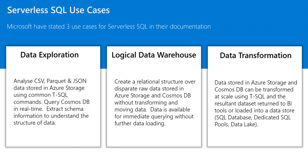
- The three main scenarios Serverless SQL can be used in which Microsoft have stated here.
- A common definition of a Logical Data Warehouse
- Describe the Serverless SQL service and its features
- Creating the first part of the Logical Data Warehouse
Parts 2 and 3 will further the concept by introducing the Data Warehouse Dimensional modelling technique to transform and load source data into a more analytical focussed format as well as incremental loading and historical analysis.
4-Part Series Link
- Creating a Logical Data Warehouse with Synapse Serverless SQL: Part 1 of 4 – Setting Up and Querying Source Data

- Creating a Logical Data Warehouse with Synapse Serverless SQL: Part 2 of 4 – Creating a Dimensional Model

- Creating a Logical Data Warehouse with Synapse Serverless SQL: Part 3 of 4 – Incremental Fact Loading and Slowly Changing Dimensions

- Creating a Logical Data Warehouse with Synapse Serverless SQL: Part 4 of 4 – Connecting Power BI to the Dimensional Model

Serverless SQL Usage Scenarios
Microsoft have stated that the Serverless SQL service can be used to create a Logical Data Warehouse to enable disparate data sources to be queried without extracting, transforming, and loading the data into another data store. The data remains in its original location and is queried “on the fly” without being moved anywhere else. This enables an organisation to extract insight from data sources without requiring additional data stores to hold transformed data.
What is a Logical Data Warehouse?
A Logical Data Warehouse is an architectural pattern that can complement a tradition data warehouse by allowing data from disparate systems to be viewed without movement or transformation. Whilst the traditional data warehouse may store a certain amount of an organisations data, a Logical Data Warehouse may enable a more holistic approach by connecting many other data sources that are not loaded into or are not appropriate to be loaded into a traditional data warehouse.
Synapse Analytics Serverless SQL Pools
The Azure Synapse Analytics SQL Serverless service enables querying file-based data stored in an Azure Storage/Data Lake Gen2 account by using familiar T-SQL. The data remains stored in the source storage account and CSV, Parquet and JSON are currently supported file types. The service enables data roles such as Data Engineers and Data Analysts to query from storage and also to write data back to storage. This service represents another tool in the Data Engineers/Data Analysts toolbox to complement the existing Dedicated SQL Pools service in that no data needs to be ingested into another data service, data can be queried in its source location in Azure Storage and the Cosmos DB service. The pricing model is based on the concept of data processed rather than time or compute tier. Data processed includes reading, writing, and metadata scanning and is currently priced around $5 per 1 Terabyte processed. Please note there is no caching available, each query will be chargeable.
In terms of using Serverless SQL to create a Logical Data Warehouse, the currently supported data sources are Azure Storage/Data Lake Gen2 and Cosmos DB. If an organisation has data stored in these services which could offer a benefit if analysed such as log and telemetry data, then Serverless SQL is an accessible service which allows leveraging of existing SQL skills.
Logical Data Warehouse Solution Walkthrough
In this section we’ll walkthrough how to create part 1 of our solution which will be to create a database in the Serverless SQL service, create connections to the underlying data lake containers and finally create views which will allow querying the source CSV file data.
Synapse Analytics Workspace Set-up
If you do not currently have an Azure Synapse Analytics Workspace setup then please follow the tutorial Getting Started with Azure Synapse Analytics SQL Serverless which will guide you through the process of setting up the service.
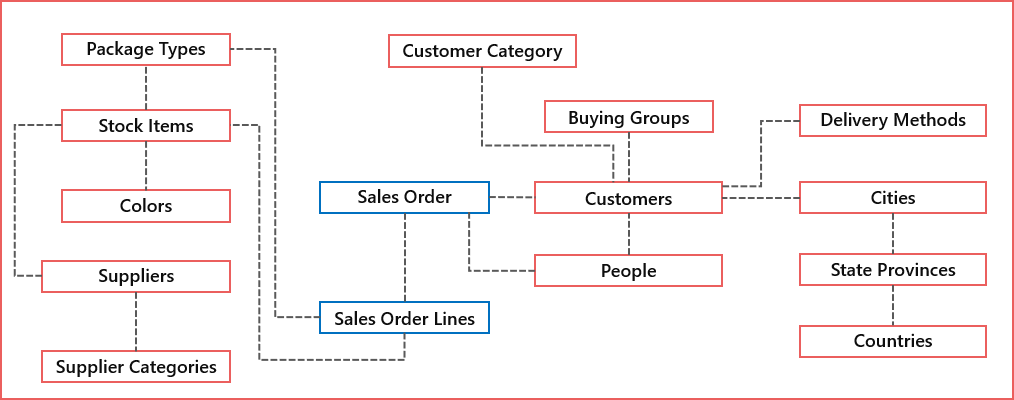
Source Data Model
For the walkthrough we’ll be using a set of tables from the WideWorldImporters example database which have been exported to CSV format. The main tables are Sales Order and Sales Order Lines with related tables including Items, Customers and Suppliers.
The CSV data is available for download here.
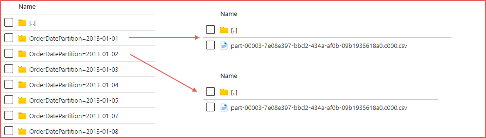
The Sales Order and Sales Order Line data comprises daily sales information across several years from 2013 to 2021. Each day of sales data is stored in a separate folder.
Recommended Practices
Throughout this blog series we’ll be ensuring, where possible, that the relevant recommended practices that Microsoft have published here are followed. These recommended practices include:
- Co-locate Storage account and Synapse Workspace: Both the Data Lake Storage account and Synapse Analytics Workspace are in the UK South region.
- Partition files within folders: Sales Orders and Sales Order Lines files are stored in date folders to allow partition pruning.
- Use PARSER_VERSION 2.0 when querying CSV files to improve read performance.
- An example of manually creating statistics to improve query performance.
- Setting data types when creating Views to ensure consistency.
- Using the filepath() function to “partition prune” and only target specific folders in the data lake to reduce data scanned and improve read performance.
Create Database and Data Sources
To begin, log into the Azure Synapse Workspace and open Synapse Studio. From the studio, click the Develop tab and create a new SQL script. All the following code is SQL so the same process of creating a SQL script in the Develop tab can be followed. The following script will create a new database in the Serverless SQL pool called sqllogicaldw create a connection to the underlying data lake storage account in Azure, creates a schema to logically store the View definition in, creates a scoped credential which uses Active Directory to authenticate with the Azure Storage account, and finally sets the collation of the database to support UTF-8 data.
CREATE DATABASE sqllogicaldw;

CREATE EXTERNAL DATA SOURCE ExternalDataSourceDataLake
	WITH (
		LOCATION   = 'https://<storageaccountname>.dfs.core.windows.net/datalakehouse'
	    );

CREATE EXTERNAL FILE FORMAT SynapseParquetFormat
WITH (
        FORMAT_TYPE = PARQUET
     );

CREATE SCHEMA LDW authorization dbo;

CREATE MASTER KEY ENCRYPTION BY PASSWORD = '<REALLY_STRING_PASSWORD!>';

CREATE DATABASE SCOPED CREDENTIAL SynapseUserIdentity
WITH IDENTITY = 'User Identity';

ALTER DATABASE sqllogicaldw COLLATE Latin1_General_100_BIN2_UTF8;
Azure Storage Authentication
As we are using “User Identity” in the database scoped credential, the user account which is being used in the Synapse Studio will need to be added to the Azure Storage Access Control (IAM) as a Storage Blob Data Contributor. Parts two and three of this blog series require data to be written to the storage account as well as read.
Azure Storage Authentication Alternative
In the SQL code above, we have used the “User Identity” option to enable pass-through authentication, however query performance can be improved using the SAS token authentication option instead. As always, testing options to find what works best in your environment is encouraged. The following code can be used to create a database scoped credential and another data source which uses the SAS token. You can create multiple database scoped credentials and data sources so feel free to create both “User Identity” and “SAS” objects and compare performance.
CREATE DATABASE SCOPED CREDENTIAL [SasToken]
WITH IDENTITY = 'SHARED ACCESS SIGNATURE',
     SECRET = '<SAS_TOKEN_FROM_STORAGE_ACCOUNT>';
GO

CREATE EXTERNAL DATA SOURCE ExternalDataSourceDataLakeSAS
WITH (    LOCATION   = 'https://storsynapsedemo.dfs.core.windows.net/datalakehouse',
          CREDENTIAL = SasToken
)
Create Views
We’ll now create Views in the Serverless SQL database to enable querying of the source data. There will be no transformation of the data at this stage except for column selection and data type assignment for certain views.
To contrast different approaches when creating the Views, in the LDW.vwSalesOrders view, we are using the HEADER_ROW = TRUE option with no explicit column selection from the underlying CSVs. In the LDW.vwSalesOrdersLines we are replacing this option with ROWSTARTS = 2 and using the WITH option to specify the column to be selected, the column names which will be used in the view, and the data type.
The Views also contain the filepath() function which is used to “partition prune” (filter) on specific folders in the data lake to minimise scanning all folders and files. This saves both time and money (amount of data processed = £££!).
CREATE VIEW LDW.vwSalesOrders
AS
SELECT *,
CAST(fct.filepath(1) AS DATE) AS FilePathDate
FROM
OPENROWSET
(
    BULK 'sourcedatapartitionsalesorder/OrderDatePartition=*/*.csv',
    DATA_SOURCE = 'ExternalDataSourceDataLake',
    FORMAT = 'CSV',
    PARSER_VERSION = '2.0',
    HEADER_ROW = TRUE,
    FIELDTERMINATOR ='|'
) AS fct

CREATE VIEW LDW.vwSalesOrdersLines
AS
SELECT *,
CAST(fct.filepath(1) AS DATE) AS FilePathDate
FROM
OPENROWSET
(
    BULK 'sourcedatapartitionsalesorderline/OrderDate=*/*.csv',
    DATA_SOURCE = 'ExternalDataSourceDataLake',
    FORMAT = 'CSV',
    PARSER_VERSION = '2.0',
    HEADER_ROW = TRUE,
    FIELDTERMINATOR ='|'
) AS fct
Data Related to Sales Orders
As there are different options when creating views in terms of column selection and data type definition, the following 4 views use different syntax to illustrate the various options available.
- LDW.vwCustomers: Uses HEADER_ROW = TRUE and SELECT *.
- LDW.vwCities: Uses HEADER_ROW = TRUE then references the CSV column names in the SELECT.
- LDW.vwStateProvinces: Uses HEADER_ROW = TRUE and the WITH statement to define column data types.
- LDW.vwCountries: Uses FIRSTROW = 2 and the WITH statement to select columns based on their ordinal position and custom column names.
CREATE VIEW LDW.vwCustomers
AS
SELECT * FROM
OPENROWSET
(
    BULK 'sourcedatasystem/Sales_Customers/*.csv',
    DATA_SOURCE = 'ExternalDataSourceDataLake',
    FORMAT = 'CSV',
    PARSER_VERSION = '2.0',
    HEADER_ROW = TRUE,
    FIELDTERMINATOR ='|'
) AS fct


CREATE VIEW LDW.vwCities
AS
SELECT CityID,
        CityName,
        StateProvinceID,
        LatestRecordedPopulation
FROM
OPENROWSET
(
    BULK 'sourcedatasystem/Application_Cities/*.csv',
    DATA_SOURCE = 'ExternalDataSourceDataLake',
    FORMAT = 'CSV',
    PARSER_VERSION = '2.0',
    HEADER_ROW = TRUE,
    FIELDTERMINATOR ='|'
) AS fct


CREATE VIEW LDW.vwStateProvinces
AS
SELECT * FROM
OPENROWSET
(
    BULK 'sourcedatasystem/Application_StateProvinces/*.csv',
    DATA_SOURCE = 'ExternalDataSourceDataLake',
    FORMAT = 'CSV',
    PARSER_VERSION = '2.0',
    HEADER_ROW = TRUE,
    FIELDTERMINATOR ='|'
)
WITH
(
    StateProvinceID TINYINT,
    StateProvinceCode CHAR(2),
    StateProvinceName VARCHAR(30),
    CountryID TINYINT,
    SalesTerritory VARCHAR(14),
    LatestRecordedPopulation INT
) AS fct


CREATE VIEW LDW.vwCountries
AS
SELECT * FROM
OPENROWSET
(
    BULK 'sourcedatasystem/Application_Countries/*.csv',
    DATA_SOURCE = 'ExternalDataSourceDataLake',
    FORMAT = 'CSV',
    PARSER_VERSION = '2.0',
    FIRSTROW = 2,
    FIELDTERMINATOR ='|'
)
WITH
(
    CountryID TINYINT 1,
    Country VARCHAR(50) 2,
    IsoCode3 CHAR(3) 4,
    CountryType VARCHAR(50) 6,
    LatestRecordedPopulation INT 7,
    Continent VARCHAR(50) 8,
    Region VARCHAR(50) 9,
    Subregion VARCHAR(50) 10
) AS fct
The remainder of the Views created will use the HEADER_ROW = TRUE syntax with SELECT * for code brevity, feel free to amend as necessary.
CREATE VIEW LDW.vwBuyingGroups
AS
SELECT * FROM
OPENROWSET
(
    BULK 'sourcedatasystem/Sales_BuyingGroups/*.csv',
    DATA_SOURCE = 'ExternalDataSourceDataLake',
    FORMAT = 'CSV',
    PARSER_VERSION = '2.0',
    HEADER_ROW = TRUE,
    FIELDTERMINATOR ='|'
) AS fct


CREATE VIEW LDW.vwDeliveryMethods
AS
SELECT * FROM
OPENROWSET
(
    BULK 'sourcedatasystem/Application_DeliveryMethods/*.csv',
    DATA_SOURCE = 'ExternalDataSourceDataLake',
    FORMAT = 'CSV',
    PARSER_VERSION = '2.0',
    HEADER_ROW = TRUE,
    FIELDTERMINATOR ='|'
) AS fct


CREATE VIEW LDW.vwCustomerCategories
AS
SELECT * FROM
OPENROWSET
(
    BULK 'sourcedatasystem/Sales_CustomerCategories/*.csv',
    DATA_SOURCE = 'ExternalDataSourceDataLake',
    FORMAT = 'CSV',
    PARSER_VERSION = '2.0',
    HEADER_ROW = TRUE,
    FIELDTERMINATOR ='|'
) AS fct


CREATE VIEW LDW.vwPeople
AS
SELECT * FROM
OPENROWSET
(
    BULK 'sourcedatasystem/Application_People/*.csv',
    DATA_SOURCE = 'ExternalDataSourceDataLake',
    FORMAT = 'CSV',
    PARSER_VERSION = '2.0',
    HEADER_ROW = TRUE,
    FIELDTERMINATOR ='|'
) AS fct
Data Related to Sales Order Lines
CREATE VIEW LDW.vwSuppliers
AS
SELECT * FROM
OPENROWSET
(
    BULK 'sourcedatasystem/Purchasing_Suppliers/*.csv',
    DATA_SOURCE = 'ExternalDataSourceDataLake',
    FORMAT = 'CSV',
    PARSER_VERSION = '2.0',
    HEADER_ROW = TRUE,
    FIELDTERMINATOR ='|'
) AS fct


CREATE VIEW LDW.vwSupplierCategories
AS
SELECT * FROM
OPENROWSET
(
    BULK 'sourcedatasystem/Purchasing_SupplierCategories/*.csv',
    DATA_SOURCE = 'ExternalDataSourceDataLake',
    FORMAT = 'CSV',
    PARSER_VERSION = '2.0',
    HEADER_ROW = TRUE,
    FIELDTERMINATOR ='|'
) AS fct


CREATE VIEW LDW.vwStockItems
AS
SELECT * FROM
OPENROWSET
(
    BULK 'sourcedatasystem/Warehouse_StockItems/*.csv',
    DATA_SOURCE = 'ExternalDataSourceDataLake',
    FORMAT = 'CSV',
    PARSER_VERSION = '2.0',
    HEADER_ROW = TRUE,
    FIELDTERMINATOR ='|'
) AS fct


CREATE VIEW LDW.vwColors
AS
SELECT * FROM
OPENROWSET
(
    BULK 'sourcedatasystem/Warehouse_Colors/*.csv',
    DATA_SOURCE = 'ExternalDataSourceDataLake',
    FORMAT = 'CSV',
    PARSER_VERSION = '2.0',
    HEADER_ROW = TRUE,
    FIELDTERMINATOR ='|'
) AS fct


CREATE VIEW LDW.vwPackageTypes
AS
SELECT * FROM
OPENROWSET
(
    BULK 'sourcedatasystem/Warehouse_PackageTypes/*.csv',
    DATA_SOURCE = 'ExternalDataSourceDataLake',
    FORMAT = 'CSV',
    PARSER_VERSION = '2.0',
    HEADER_ROW = TRUE,
    FIELDTERMINATOR ='|'
) AS fct
Querying Source Data Views
Now that the base views are in place to SELECT from the source CSV data, we can query these views to return useful aggregations.
Aggregate Queries
SELECT YEAR(SO.OrderDate) AS OrderDateYear,
        COUNT(SO.OrderDate) AS TotalOrderCount
FROM LDW.vwSalesOrders SO
GROUP BY YEAR(SO.OrderDate);

SELECT ISNULL(C.ColorName,'No Colour') AS ColourName,
    SUM(SOL.Quantity) AS TotalOrderLineQuantity,
    SUM(SOL.UnitPrice) AS TotalOrderLineUnitPrice
FROM LDW.vwSalesOrdersLines SOL
INNER JOIN LDW.vwStockItems SI ON SI.StockItemID = SOL.StockItemID
LEFT JOIN LDW.vwColors C ON C.ColorID = SI.ColorID
GROUP BY ISNULL(C.ColorName,'No Colour');

SELECT
    YEAR(SO.OrderDate) AS OrderDateYear,
    SC.SupplierCategoryName,
    SUM(SOL.Quantity) AS TotalOrderLineQuantity,
    SUM(SOL.UnitPrice) AS TotalOrderLineUnitPrice
FROM LDW.vwSalesOrdersLines SOL
INNER JOIN LDW.vwSalesOrders SO ON SO.OrderID = SOL.OrderID
INNER JOIN LDW.vwStockItems SI ON SI.StockItemID = SOL.StockItemID
INNER JOIN LDW.vwSuppliers S ON SI.SupplierID = S.SupplierID
INNER JOIN LDW.vwSupplierCategories SC ON SC.SupplierCategoryID = S.SupplierCategoryID
GROUP BY YEAR(SO.OrderDate),
        SC.SupplierCategoryName;
Filtering and Manual Statistics Creation
We can filter the data, however the following query will filter based on the OrderDate column but Serverless SQL will scan all the underlying folders and files.
SELECT COUNT(SO.OrderID) AS TotalOrderCount
FROM LDW.vwSalesOrders SO
WHERE SO.OrderDate = '2017-02-16'
We can manually create statistics on the OrderDate column to improve query performance.
EXEC sys.sp_create_openrowset_statistics N'
    SELECT OrderDate
FROM
OPENROWSET
(
    BULK ''sourcedatapartitionsalesorder/*/*.csv'',
    DATA_SOURCE = ''ExternalDataSourceDataLake'',
    FORMAT = ''CSV'',
    PARSER_VERSION = ''2.0'',
    HEADER_ROW = TRUE,
    FIELDTERMINATOR =''|''
) AS fct
'
Pushing Filters down to the Folder
We can use the filepath() function to only scan the required folder in the data lake and therefore reduce the amount of data scanned.
SELECT YEAR(SO.OrderDate) AS OrderDateYear,
        COUNT(SO.OrderDate) AS TotalOrderCount
FROM LDW.vwSalesOrders SO
WHERE SO.FilePathDate = '2017-02-16'
GROUP BY YEAR(SO.OrderDate)
Creating Views for Analytical Queries
We can now create Views to join these source data views together to start answering reporting/analytical questions such as “how many Sales Orders were placed for certain Stock Items”.
CREATE VIEW LDW.vwDimStockItems
AS
SELECT  SI.StockItemID,
        SI.StockItemName,
        SI.LeadTimeDays,
        SI.TaxRate,
        SI.UnitPrice,
        SI.SearchDetails,
        PTUnit.PackageTypeName AS PackageTypeNameUnit,
        PTOut.PackageTypeName AS PackageTypeNameOuter,
        C.ColorName,
        S.SupplierName,
        S.PaymentDays,
        SC.SupplierCategoryName
FROM LDW.vwStockItems SI
LEFT JOIN LDW.vwPackageTypes PTUnit ON PTUnit.PackageTypeID = SI.UnitPackageID
LEFT JOIN LDW.vwPackageTypes PTOut ON PTOut.PackageTypeID = SI.OuterPackageID
LEFT JOIN LDW.vwColors C ON C.ColorID = SI.ColorID
LEFT JOIN LDW.vwSuppliers S ON S.SupplierID = SI.SupplierID
LEFT JOIN LDW.vwSupplierCategories SC ON SC.SupplierCategoryID = S.SupplierCategoryID
CREATE VIEW LDW.vwDimCustomers
AS
SELECT  C.CustomerID,
        C.CustomerName,
        C.AccountOpenedDate,
        C.CreditLimit,
        C.PaymentDays,
        CT.CityName AS CityNameDelivery,
        SP.StateProvinceCode AS StateProvinceCodeDelivery,
        SP.StateProvinceName AS StateProvinceNameDelivery,
        SP.SalesTerritory AS SalesTerritoryDelivery,
        CR.Country AS CountryDelivery,
        CR.Continent AS ContinentDelivery,
        CR.Region AS RegionDelivery,
        CR.Subregion AS SubregionDelivery,
        P.FullName AS PrimaryContactPersonName,
        CC.CustomerCategoryName,
        BG.BuyingGroupName,
        DM.DeliveryMethodName
FROM LDW.vwCustomers C
LEFT JOIN LDW.vwCities CT ON CT.CityID = C.DeliveryCityID
LEFT JOIN LDW.vwStateProvinces SP ON SP.StateProvinceID = CT.StateProvinceID
LEFT JOIN LDW.vwCountries CR ON CR.CountryID = SP.CountryID
LEFT JOIN LDW.vwPeople P ON P.PersonID = C.PrimaryContactPersonID
LEFT JOIN LDW.vwCustomerCategories CC ON CC.CustomerCategoryID = C.CustomerCategoryID
LEFT JOIN LDW.vwBuyingGroups BG ON BG.BuyingGroupID = C.BuyingGroupID
LEFT JOIN LDW.vwDeliveryMethods DM ON DM.DeliveryMethodID = C.DeliveryMethodID
Using Analytical Views
Now that we have 2 Views that have “denormalised” the source data, we can now use these views to join to the Sales Order and Sales Order Line views.
SELECT DC.CustomerCategoryName,
        DS.PackageTypeNameUnit,
        SUM(SOL.Quantity) AS TotalOrderLineQuantity,
        SUM(SOL.UnitPrice) AS TotalOrderLineUnitPrice
FROM LDW.vwSalesOrdersLines SOL
INNER JOIN LDW.vwSalesOrders SO ON SO.OrderID = SOL.OrderID
INNER JOIN LDW.vwDimCustomers DC ON DC.CustomerID = SO.CustomerID
INNER JOIN LDW.vwDimStockItems DS ON DS.StockItemID = SOL.StockItemID
GROUP BY DC.CustomerCategoryName,
        DS.PackageTypeNameUnit
Conclusion
In this blog post, part one of three, we have set-up a Synapse Workspace, created a new database, then created views to query the source CSV data. In part 2 we will look at writing data back to the data lake using CETAS (Create External Table As Select) and storing data using the parquet file format for more performant data retrieval.
 Andy
Andy