

Welcome to part 2 of this 4 part blog series on creating a Logical Data Warehouse with Azure Synapse Analytics Serverless SQL. Please note that we are only using Serverless SQL Pools, other Synapse Analytics services such as Pipelines/Dedicated SQL Pools/Spark Pools are out of scope.
In part one we went through the process of connecting to source data in CSV format and creating Views in a new Serverless SQL Pools database to query this data. During this process no data was actually transformed or moved from its source location in Azure Storage. Whilst this is certainly a benefit and a fundamental concept of the Logical Data Warehouse architecture, there may be instances where transforming and saving this data may be preferable. In part 2 we’ll be transforming the source CSV data into a “de-normalised” dimensional format better suited for reporting and analytical queries. However we will still be using Azure Storage to write the transformed data to by using Serverless SQL Pools.
All SQL code is available on GitHub.
4-Part Series Link
- Creating a Logical Data Warehouse with Synapse Serverless SQL: Part 1 of 4 – Setting Up and Querying Source Data

- Creating a Logical Data Warehouse with Synapse Serverless SQL: Part 2 of 4 – Creating a Dimensional Model

- Creating a Logical Data Warehouse with Synapse Serverless SQL: Part 3 of 4 – Incremental Fact Loading and Slowly Changing Dimensions

- Creating a Logical Data Warehouse with Synapse Serverless SQL: Part 4 of 4 – Connecting Power BI to the Dimensional Model

Using CETAS to write data to the Data Lake
So far we have used Serverless SQL Pools to read data from Azure Storage, now we will use the CETAS process to write data back to the data lake. This CETAS process is the CREATE EXTERNAL TABLE AS SELECT (CETAS) syntax and allows us to write data to Azure Storage from a SELECT statement.
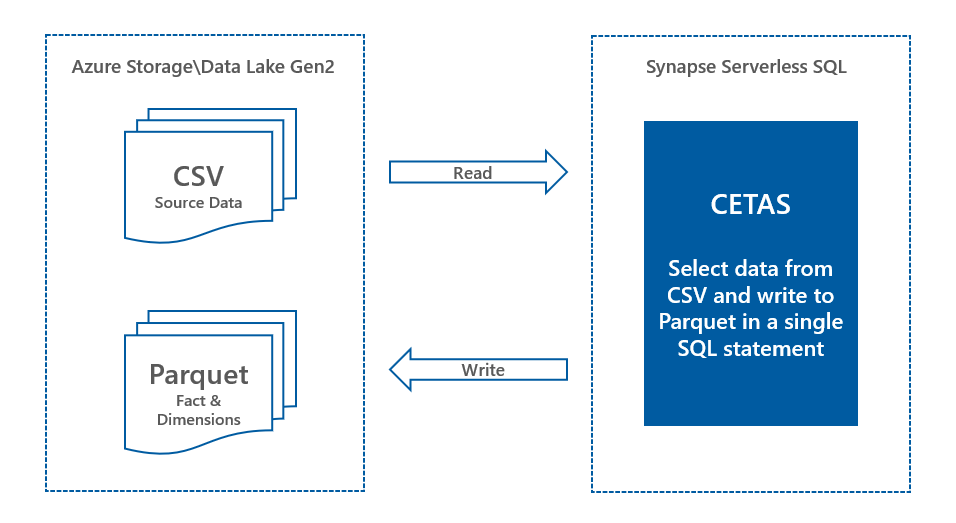
In this scenario we will use the CETAS statement to create an External Table to load the source CSV data and save into the Parquet file format. We are using the creation of an external table as a loading mechanism, to read this data we will create Views. In fact, the external table can be dropped once the statement has completed as the newly-written data is not deleted.
Introducing the Parquet file format
Parquet is a columnar file format which stores the data, the schema information including column names and data types, and also statistics about the data. It supports predicate pushdown meaning only those columns and row data required to satisfy the SQL query issued are returned. Compare that to CSV which requires the entire CSV file to be processed/read regardless of which columns are selected and any filters used. However, Parquet is not readable using a text editor like CSV and JSON.
As Parquet improves performance in terms of reading file-based data from data lakes and also reduces the amount of data stored and processed, it is a preferable format for data analytics projects.
Dimensional Modelling and the Star Schema
Why are we using a Star Schema? This has been a mainstay of Data Warehousing for many years and remains as relevant today as when the concept was first introduced. The process of constructing a Star Schema involves dimensional modelling, which is a process to identify what you want to measure (Facts) and how you want to measure (Dimensions). The process takes an organisation through a thought-provoking exercise to identify this information.
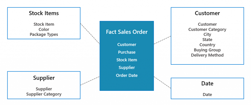
The Dimensional model for our example project comprises of 1 Fact table and 4 Dimension tables.
Creating Dimensions
We’ll begin by creating 4 dimensions, 3 of these dimensions will be created by joining several relevant source views together whilst the Date dimension will be created from a single source file.
Surrogate Keys
Microsoft recommended practices state using integers can improve query performance. Currently our test solution “business keys” (primary keys in the source data) are mostly integer-based except date, which is converted to an integer. However, there could be a situation where the source data has character/alpha-numeric primary keys and therefore impact and join and filter performance and could increase data processed costs. Ideally we need to ensure the space used by our data types are minimised as much as possible.
Using CETAS to write source data as Parquet
We’ll now use CETAS to write the source data to a destination folder. Please note the following:
- The load will write the data out to a sub-folder \01\ in each dimension (except the Date dimension) as this is the initial load. Future loads will populate a sequence of sub-folders.
- We use ROW_NUMBER() to generate a surrogate key on type Integer.
- A ValidFromDate of 2013-01-01 is used as this is the start of our Sales data.
- Data quality checking such as NULL attributes are currently not being dealt with in this solution for the sake of code brevity.
CREATE SCHEMA STG AUTHORIZATION dbo;

--Create Parquet file format
CREATE EXTERNAL FILE FORMAT SynapseParquetFormat
WITH (
        FORMAT_TYPE = PARQUET
     );

--Customer
CREATE EXTERNAL TABLE STG.DimCustomer
WITH
(
  LOCATION = 'conformed/dimensions/dimcustomer/01',
  DATA_SOURCE = ExternalDataSourceDataLake,
  FILE_FORMAT = SynapseParquetFormat
)
AS
SELECT CAST(ROW_NUMBER() OVER(ORDER BY C.CustomerID) AS INT) AS CustomerKey,
        CAST(C.CustomerID AS INT) AS CustomerID,
        C.CustomerName,
        CC.CustomerCategoryName,
        BG.BuyingGroupName,
        DM.DeliveryMethodName,
        DC.CityName AS DeliveryCityName,
        DSP.StateProvinceName AS DeliveryStateProvinceName,
        DSP.SalesTerritory AS DeliverySalesTerritory,
        DCO.Country AS DeliveryCountry,
        DCO.Continent AS DeliveryContinent,
        DCO.Region AS DeliveryRegion,
        DCO.Subregion AS DeliverySubregion,
        CAST('2013-01-01' AS DATE) AS ValidFromDate
FROM LDW.vwCustomers C
LEFT JOIN LDW.vwCustomerCategories CC On CC.CustomerCategoryID = C.CustomerCategoryID
LEFT JOIN LDW.vwCities DC ON DC.CityID = C.DeliveryCityID
LEFT JOIN LDW.vwStateProvinces DSP ON DSP.StateProvinceID = DC.StateProvinceID
LEFT JOIN LDW.vwCountries DCO ON DCO.CountryID = DSP.CountryID
LEFT JOIN LDW.vwBuyingGroups BG ON BG.BuyingGroupID = C.BuyingGroupID
LEFT JOIN LDW.vwDeliveryMethods DM ON DM.DeliveryMethodID = C.DeliveryMethodID
ORDER BY C.CustomerID

--StockItem
CREATE EXTERNAL TABLE STG.DimStockItem
WITH
(
  LOCATION = 'conformed/dimensions/dimstockitem/01',
  DATA_SOURCE = ExternalDataSourceDataLake,
  FILE_FORMAT = SynapseParquetFormat
)
AS
SELECT CAST(ROW_NUMBER() OVER(ORDER BY SI.StockItemID) AS SMALLINT) AS StockItemKey,
CAST(SI.StockItemID AS SMALLINT) AS StockItemID,
SI.StockItemName,
SI.LeadTimeDays,
C.ColorName,
OP.PackageTypeName AS OuterPackageTypeName,
CAST('2013-01-01' AS DATE) AS ValidFromDate
FROM LDW.vwStockItems SI
LEFT JOIN LDW.vwColors C ON C.ColorID = SI.ColorID
LEFT JOIN LDW.vwPackageTypes OP ON OP.PackageTypeID = SI.OuterPackageID
ORDER BY SI.StockItemID

--Supplier
CREATE EXTERNAL TABLE STG.DimSupplier
WITH
(
  LOCATION = 'conformed/dimensions/dimsupplier/01',
  DATA_SOURCE = ExternalDataSourceDataLake,
  FILE_FORMAT = SynapseParquetFormat
)
AS
SELECT CAST(ROW_NUMBER() OVER(ORDER BY S.SupplierID) AS TINYINT) AS SupplierKey,
CAST(S.SupplierID AS TINYINT) AS SupplierID,
S.SupplierName,
SC.SupplierCategoryName,
CAST('2013-01-01' AS DATE) AS ValidFromDate
FROM LDW.vwSuppliers S
LEFT JOIN LDW.vwSupplierCategories SC ON SC.SupplierCategoryID = S.SupplierCategoryID
ORDER BY S.SupplierID;

--Date
CREATE EXTERNAL TABLE STG.DimDate
WITH
(
  LOCATION = 'conformed/dimensions/dimdate',
  DATA_SOURCE = ExternalDataSourceDataLake,
  FILE_FORMAT = SynapseParquetFormat
)
AS
SELECT CAST(DateKey AS INT) AS DateKey,
        CAST(Date AS DATE) AS Date,
        CAST(Day AS TINYINT) AS Day,
        CAST(WeekDay AS TINYINT) AS WeekDay,
        WeekDayName,
        CAST(Month AS TINYINT) AS Month,
        MonthName,
        CAST(Quarter AS TINYINT) AS Quarter,
        CAST(Year AS SMALLINT) AS Year
FROM
OPENROWSET
(
    BULK 'sourcedatadim/datedim/*.csv',
    DATA_SOURCE = 'ExternalDataSourceDataLake',
    FORMAT = 'CSV',
    PARSER_VERSION = '2.0',
    HEADER_ROW = TRUE,
    FIELDTERMINATOR ='|'
) AS fct
Create Views for Dimensions
We now create Views on the newly written Parquet data. The primary reason for this is that further data can be written to different folders under the specific dimension folder. This is addressed in the 3rd part of this blog series.
In Part 1 we created 2 Views to mimic dimensions, we will drop these views before creating the new Views.
DROP VIEW LDW.vwDimCustomers;
DROP VIEW LDW.vwDimStockItems;
--Customer
CREATE VIEW LDW.vwDimCustomer
AS
SELECT * FROM
OPENROWSET
(
BULK 'conformed/dimensions/dimcustomer/*/',
DATA_SOURCE = 'ExternalDataSourceDataLake',
FORMAT = 'Parquet'
) AS fct
--StockItem
CREATE VIEW LDW.vwDimStockItem
AS
SELECT * FROM
OPENROWSET
(
BULK 'conformed/dimensions/dimstockitem/*/',
DATA_SOURCE = 'ExternalDataSourceDataLake',
FORMAT = 'Parquet'
) AS fct
--Supplier
CREATE VIEW LDW.vwDimSupplier
AS
SELECT * FROM
OPENROWSET
(
BULK 'conformed/dimensions/dimsupplier/*/',
DATA_SOURCE = 'ExternalDataSourceDataLake',
FORMAT = 'Parquet'
) AS fct
--Date
CREATE VIEW LDW.vwDimDate
AS
SELECT * FROM
OPENROWSET
(
BULK 'conformed/dimensions/dimdate',
DATA_SOURCE = 'ExternalDataSourceDataLake',
FORMAT = 'Parquet'
) AS fctCreating Facts
In this scenario we’ll create a single Fact table from the source Sales Order and Sales Order Detail data with a link to all dimensions. As the Sales Order (header) data does not contain any information that must be split out across multiple Sales Order Detail lines such as shipping amounts, we will model our data by taking any header attributes down into the detail.
We could model our Facts as separate “Header” and “Line” to remove any DISTINCT operations on the Sales Order count but for this scenario we will model as a single Fact.
CREATE EXTERNAL TABLE STG.FactSales
WITH
(
  LOCATION = 'conformed/facts/factsales/initial',
  DATA_SOURCE = ExternalDataSourceDataLake,
  FILE_FORMAT = SynapseParquetFormat
)
AS
SELECT
  --Surrogate Keys
    DC.CustomerKey,
    CAST(FORMAT(SO.OrderDate,'yyyyMMdd') AS INT) as OrderDateKey,
    DSI.StockItemKey,
    DS.SupplierKey,
    --Degenerate Dimensions
    CAST(SO.OrderID AS INT) AS OrderID,
    CAST(SOL.OrderLineID AS INT) AS OrderLineID,
    --Measure
    CAST(SOL.Quantity AS INT) AS SalesOrderQuantity,
    CAST(SOL.UnitPrice AS DECIMAL(18,2)) AS SalesOrderUnitPrice
FROM LDW.vwSalesOrdersLines SOL
INNER JOIN LDW.vwSalesOrders SO ON SOL.OrderID = SO.OrderID
LEFT JOIN LDW.vwDimCustomer DC ON DC.CustomerID = SO.CustomerID
LEFT JOIN LDW.vwDimStockItem DSI ON DSI.StockItemID = SOL.StockItemID
LEFT JOIN LDW.vwStockItems SI ON SI.StockItemID = DSI.StockItemID
LEFT JOIN LDW.vwDimSupplier DS ON DS.SupplierID = SI.SupplierID;
Create View for Facts
As we did for the Dimensions, we will also create a View over the newly-written Parquet data.
CREATE VIEW LDW.vwFactSales
AS
SELECT * FROM
OPENROWSET
(
    BULK 'conformed/facts/factsales/initial',
    DATA_SOURCE = 'ExternalDataSourceDataLake',
    FORMAT = 'Parquet'
) AS fct
Attempting to write to a folder that already exists
If a CETAS operation is attempted on a folder that already exists, for example writing out the Sales Orders has already been completed but another attempt is made, the operation will fail due to the folder already existing. Now, this means that duplicate data cannot be written out to the folder which is a benefit, however if you need to write out a new version of the data then the folder (and contents) will need to be deleted before another CETAS operation can be attempted. You do this by issuing the DROP EXTERNAL TABLE… command then deleting the newly-created folder.
Using the Dimension and Fact Views for Analysis
Once our Dimension and Fact data has been written in Parquet format using the CETAS process and new Views created to read this data, we can now use the Dimension and Fact views to query the sales data.
--Group Sales by Date
SELECT DD.[Year] AS SalesYear,
    DD.[Month] AS SalesMonth,
SUM(FS.Quantity) AS SalesOrderQuantity,
SUM(FS.UnitPrice) AS SalesOrderUnitPrice,
COUNT(DISTINCT FS.OrderID) AS SalesOrderTotal
FROM LDW.vwFactSales FS
INNER JOIN LDW.vwDimDate DD ON DD.DateKey = FS.OrderDateKey
GROUP BY DD.[Year],
         DD.[Month]
ORDER BY DD.[Year],
         DD.[Month];

--Group Sales by Customer
SELECT DC.DeliverySalesTerritory,
SUM(FS.Quantity) AS SalesOrderQuantity,
SUM(FS.UnitPrice) AS SalesOrderUnitPrice,
COUNT(DISTINCT OrderID) AS SalesOrderTotal
FROM LDW.vwFactSales FS
INNER JOIN LDW.vwDimCustomer DC ON DC.CustomerKey = FS.CustomerKey
GROUP BY DC.DeliverySalesTerritory
ORDER BY SUM(FS.Quantity) DESC;

--Group Sales by Supplier
--Note that multiple Suppliers can be linked to a single Sales Order
SELECT DS.SupplierName,
SUM(FS.Quantity) AS SalesOrderQuantity,
SUM(FS.UnitPrice) AS SalesOrderUnitPrice
FROM LDW.vwFactSales FS
INNER JOIN LDW.vwDimSupplier DS ON DS.SupplierKey = FS.SupplierKey
GROUP BY DS.SupplierName
ORDER BY SUM(FS.Quantity) DESC;
Checking Data Types
We can also check the data types that have been created, perhaps there is further optimisation available by re-writing the data and using more efficient data types.
EXEC sp_describe_first_result_set N'SELECT * FROM LDW.vwDimDate';

EXEC sp_describe_first_result_set N'SELECT * FROM LDW.vwDimSupplier';

EXEC sp_describe_first_result_set N'SELECT * FROM LDW.vwDimStockItem';

EXEC sp_describe_first_result_set N'SELECT * FROM LDW.vwDimCustomer';

EXEC sp_describe_first_result_set N'SELECT * FROM LDW.vwFactSales';
Conclusion
In part 2, we have enhanced our Logical Data Warehouse by loading data from the source CSV, de-normalising the source data as Dimensions, creating facts with surrogate keys, and saving into Parquet file format. By loading the source CSV data in Parquet, we have transformed the source data into a more efficient analytical structure.
Part 3 will conclude this blog series and will focus on incremental loading of Facts and a Slowly-Changing Dimension pattern to track changing source data attributes.
 Andy
Andy